A grand goal in deep learning research is to learn representations capable of generalizing across distribution shifts. Disentanglement is one promising direction aimed at aligning a models representations with the underlying factors generating the data (e.g. color or background). Existing disentanglement methods, however, rely on an often unrealistic assumption - that factors are statistically independent. In reality, factors (like object color and shape) are correlated. To address this limitation, we propose a relaxed disentanglement criterion - the Hausdorff Factorized Support (HFS) criterion - that encourages a factorized support, rather than a factorial distribution, by minimizing a Hausdorff distance. This allows for arbitrary distributions of the factors over their support, including correlations between them. We show that the use of HFS consistently facilitates disentanglement and recovery of ground-truth factors across a variety of correlation settings and benchmarks, even under severe training correlations and correlation shifts, with in parts over +60% in relative improvement over existing disentanglement methods. In addition, we find that leveraging HFS for representation learning can even facilitate transfer to downstream tasks such as classification under distribution shifts. We hope our original approach and positive empirical results inspire further progress on the open problem of robust generalization.
Introduction
Disentangled representation learning is a promising path to facilitate reliable generalization to in- and out-of-distribution downstream tasks, on top of being more interpretable and fair (Bengio et al. 2013, Higgins et al. 2018, Locatello et al. 2019,2020). While various metrics have been proposed to measure disentanglement, the most commonly understood definition is as follows:
Definition. Assuming the data has been generated by a set of unknown, ground-truth latent factors, a representation is said to be disentangled if each factor is recovered in one and only one dimension of the representation.
The method by which to achieve this goal however, remains an open research question. Weak and semi-supervised settings, e.g. using paired data samples or auxiliary variables, can provably offer disentanglement and recovery of ground truth factors (e.g. Bouchacourt et al. 2018, Locatello et al. 2020, ...). But fully unsupervised disentanglement -- our focus in this study -- is in theory impossible to achieve in the general unconstrained nonlinear case (c.f. Hyvaerinen et al. 1999, Locatello et al. 2019). In practice however, the inductive biases embodied in common autoencoder architectures allow for effective practical disentanglement (Rolinek et al. 2019).
Perhaps more problematic, standard unsupervised disentanglement methods (s.a. -(TC)VAE, AnnealedVAE, DIP-VAE, ...) rely on an unrealistic assumption of statistical independence of ground truth factors. Real data however contains correlations (Traeuble et al. 2021). Even with well defined factors, such as object shape, color or background, correlations are pervasive: yellow bananas are more frequent than red ones; and cows are much more often on pasture than sand dunes. In more realistic settings where factors are correlated, prior work has shown existing disentanglement methods fail.
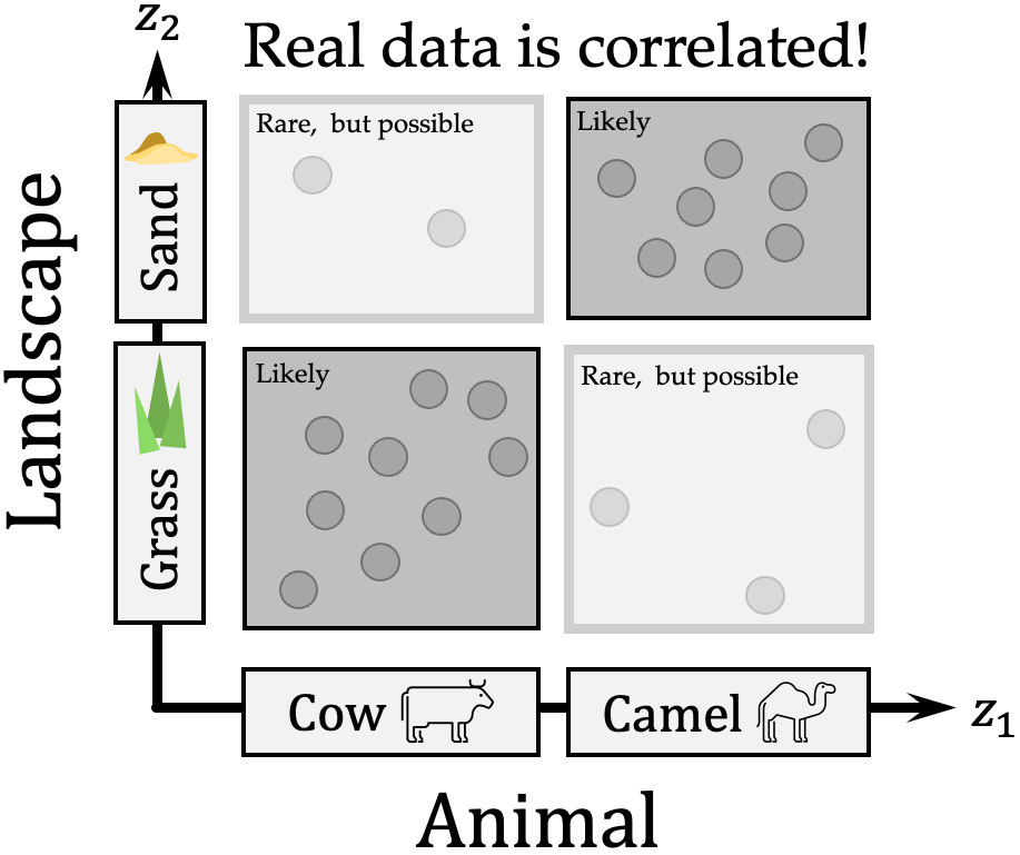
To address this limitation, we propose to relax the unrealistic assumption of statistical independence of factors (i.e. that they have a factorial distribution), and only assume the support of the factors' distribution factorizes -- a much weaker, but more realistic constraint. To visualize this, consider a dataset of animal images where background and animal type are heavily correlated (camels most likely on sand, and cows on grass):

Under the original assumption of factor independence, a model likely learns a shortcut solution where animal and landscape share the same latent correspondence (Beery et al. 2018). On the other hand with a factorized support, learned factors should be such that any combination of their values has some grounding in reality: a cow on sand is an unlikely, yet not impossible combination. We still rely, just as standard unsupervised disentanglement methods, on the inductive bias of encoder-decoder architectures to recover factors -- however, we expect our method to facilitate robustness to any distribution shifts within the support, as it makes no assumptions on the distribution beyond its factorized support.
Method
On this basis, we propose a concrete pairwise Hausdorff Factorized Support (HFS) training criterion to disentangle correlated factors, by aiming for all pairs of latents to have a factorized support. Specifically, we encourage a factorized support by minimizing a Hausdorff set-distance between the finite sample approximation of the actual support and its factorization (c.f. Huttenlocher et al. 1993, Rockafellar et al. 1998).
Setup.
To explain, we first describe the general setting: We are given a dataset (e.g. images), where each is a realization of a random variable, e.g., an image. We consider that each is generated by an unknown generative process, involving a ground truth latent random vector whose components correspond to the dataset's underlying factors of variations (s.a. object shape, color, background, \ldots). This process generates an observation , by first drawing a realization from a distribution , i.e. . Observation is then obtained by drawing .
Given , the goal of disentangled representation learning can be stated as learning a mapping that for any recovers as best as possible the associated i.e. up to a permutation of elements and elementwise bijective transformation.
Statistical Independence.
In unsupervised disentanglement, the are unobserved, and both and are a priori unknown to us, though we might assume specific properties and functional forms.
Most unsupervised disentanglement methods follow the formalization of VAEs and employ parameterized probabilistic generative models of the form to estimate the ground truth generative model over . As in VAEs, these methods make the strong assumption that ground truth factors are statistically independent,
and conflate the goal of learning a disentangled representation with that of learning a representation with statically independent components. This assumption naturally translates to a factorial model prior .
Factorized Support.
Instead of assuming independent factors (i.e. a factorial distribution on as noted above), we will only assume that the support of the distribution factorizes. Let us denote by the support of , i.e. the set . We say that is factorized if it equals to the Cartesian product of supports over individual dimensions' marginals, i.e. if:
where denotes the Cartesian product.
Of course, independence implies a factorized support, but not the other way - assuming a factorized support is thus a relaxation of the (unrealistic) assumption of factorial distribution, i.e. statistical independence of disentangled factors. Refer to the previous cartoon example, where the distribution of the two disentangled factors would not satisfy an independence assumption, but does have a factorized support. Informally the factorized support assumption is merely stating that whatever values and , etc... may take individually, any combination of these is possible (even when not very likely).
Basic Hausdorff Factorization Objective.
For our objective, let us consider deterministic representations obtained by some encoder . We enforce the factorial support criterion on the aggregate distribution , where is conceptually similar to the aggregate posterior in e.g. -TCVAE, though we consider points produced by a deterministic mapping rather than a stochastic one.
To now encourage support factorization, we now need some divergence or metric to tell us how far our encoder support is from . Supports are sets, so it is natural to use a set distance such as the Hausdorff distance, giving
with the second part of the Hausdorff distance equating to zero since .
Practical Implementation.
In practial settings with a finite sample of observations , we further introduce a practical Monte-Carlo batch-approximation: with access to a batch of inputs yielding -dimensional latent representations , we estimate Hausdorff distances using sample-based approximations to the support:
Here must be understood as the set (not vector) of all elements in the column of . Plugging into above equation yields:
where by noting we consider the matrix as a set of rows.
Sliced Hausdorff Factorized Support.
In high dimension, with many factors, the assumption that every combination of all latent values is possible might still be too strong an assumption. And even if we assumed all to be in principle possible, we can never hope to observe all in a finite dataset of realistic size due to the combinatorial explosion of conceivable combinations. However, it is statistically reasonable to expect evidence of a factorized support for all pairs of elements. To encourage such a pairwise factorized support, we minimize a sliced, pairwise Hausdorff estimate with the additional benefit of keeping computation tractable when is large:
where denotes the concatenation of column and column , yielding again a set of rows.
Final objective: avoiding collapse and retaining input information.
We will be learning representations by learning parameters that optimize a training objective. Because the Hausdorff distance builds on a base distance , if we were to minimize only this, it could be trivially minimized to 0 by collapsing all representations to a single point. Avoiding this can be achieved in several ways, s.a. by including a term that encourages the variance of to be above 1 (a technique used e.g. in self-supervised learning method VICReg \citep{bardes2022vicreg}) or -- more in line with traditional VAE variants for disentanglement -- by using a stochastic autoencoder (SAE) reconstruction error:
where typically with mean given by our deterministic mapping , producing a diagonal covariance parameter, and e.g. with a parameterized decoder. The autoencoder term ensures representations retaining as much information as possible about for reconstruction, preventing collapse of representations to a single point. A minimum scale can also be ensured by imposing by construction to be above a minimal threshold.
Consequently, this gives a standard HFS objective:
or, alternatively, one may also leverage HFS as a regularizer alongside other disentanglement methods to reliably improve disentanglement - focusing more on support factorization than statistical independence, but being able to leverage it when possible (since there may also be pairs for which statistical independence is a suitable assumption).
Experiments
Across large-scale experiments on standard disentanglement benchmarks and novel extensions with correlated factors, HFS consistently facilitates disentanglement.
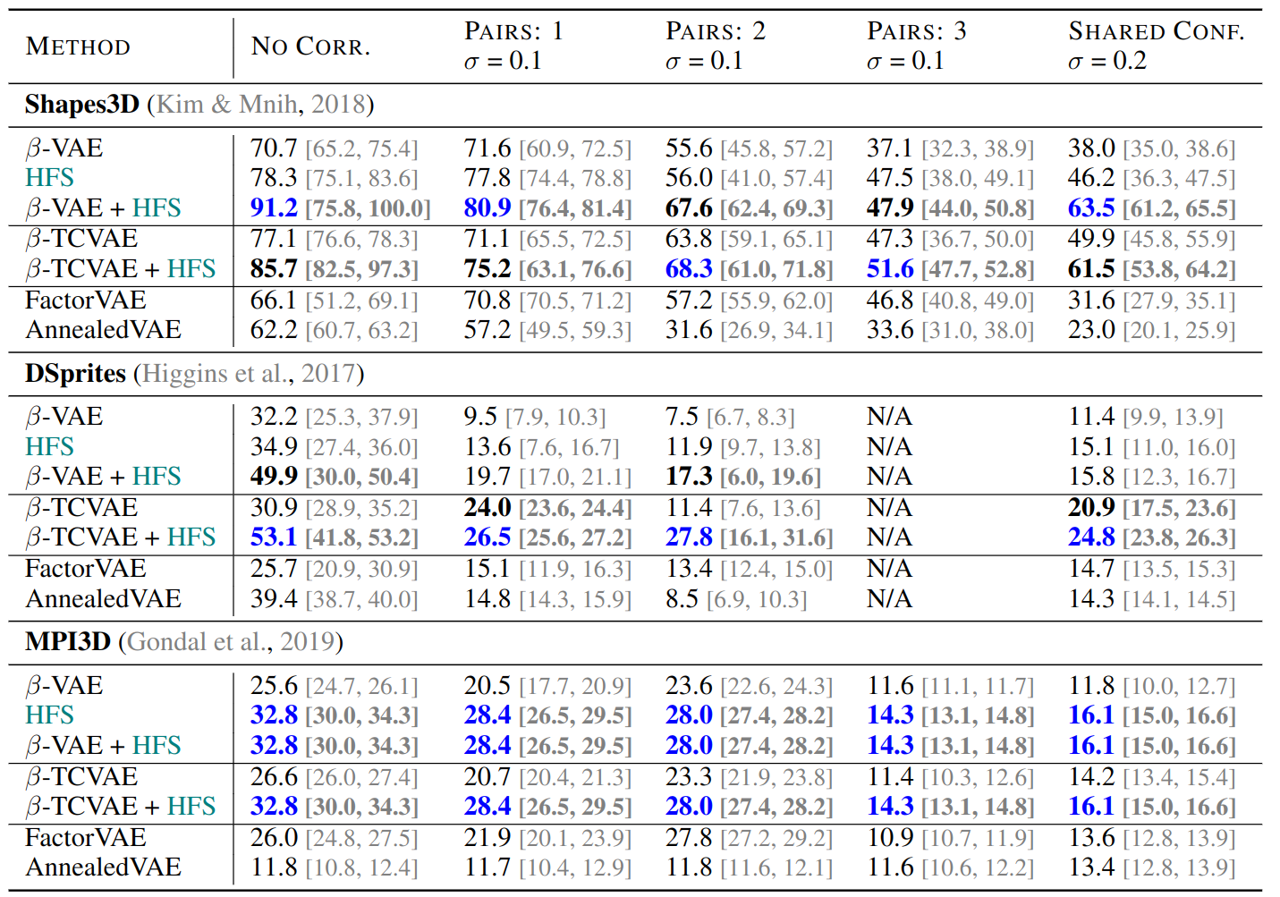
To begin, we first create various benchmarks that introduce increasingly more difficult artificial correlations between ground-truth factors. Specifically, given two ground truth factors and , we set their joint sampling probability as
This means that for lower scaling values , we get stronger correlations between factors, which we can also extend to multiple pairings. Doing so for multiple different benchmark datasets, and running existing disentanglement methods both with and without HFS regularization, as well as HFS as a standalone objective, shows significant improvements of in parts over in disentanglement performance over baselines as measured by DCI-D (Eastwood et al. 2018):

This provides strong evidence towards the benefits of focusing on support factorization over hard statistical independence. Going even further, we now introduce an even larger range of possible training correlation. In addition, correlations are introduced in the test data as well, which allows us to produce artifical distribution shifts between training and testing that we can evaluate our model on. In doing so, we interestingly find that leveraging support factorization can provide increased generalization benefits for harder out-of-distribution shifts:

Finally, another interesting benefit is the fact that the significantly increased degree of unsupervised disentanglement also results in increased adaptation speeds when training a gradient-boosted decision tree on representations over increasingly reduced amounts of training data:

Conclusion
To avoid the unrealistic assumption of factors independence (i.e. factorial distribution) as in traditional disentanglement, which stands in contrast to realistic data being correlated, we thoroughly investigate an approach that only aims at recovering a factorized support. Doing so achieves disentanglement by ensuring the model can encode many possible combinations of generative factors in the learned latent space, while allowing for arbitrary distributions over the support -- in particular those with correlations. Indeed, through a practical criterion using pairwise Hausdorff set-distances -- HFS -- we show that encouraging a pairwise factorized support is sufficient to match traditional disentanglement methods. Furthermore we show that HFS can steer existing disentanglement methods towards a more factorized support, giving large relative improvements of over on common benchmarks across a large variety of increasingly harder correlation shifts. We find this improvement in disentanglement across correlation shifts to be also reflected in improved out-of-distribution generalization especially as these shifts become more severe; tackling a key promise for disentangled representation learning.